Note: The data used in today’s posting is from the extracted MLP parameter weights of yesterday.
The Jupyter Notebook for this little project is found here.
Inspecting the ANN model parameters
After loading the model parameters, we begin to look at (1) how many parameters are there and (2) what is the structure of these parameters.
Number of params: 4
-------------------
(784, 100)   # Weights for input to hidden layer
(100,)       # Bias weights to hidden layer
(100, 10)    # Weights for hidden to output layer
(10,)        # Bias weights to output layer
Visualizing parameter weights between layers
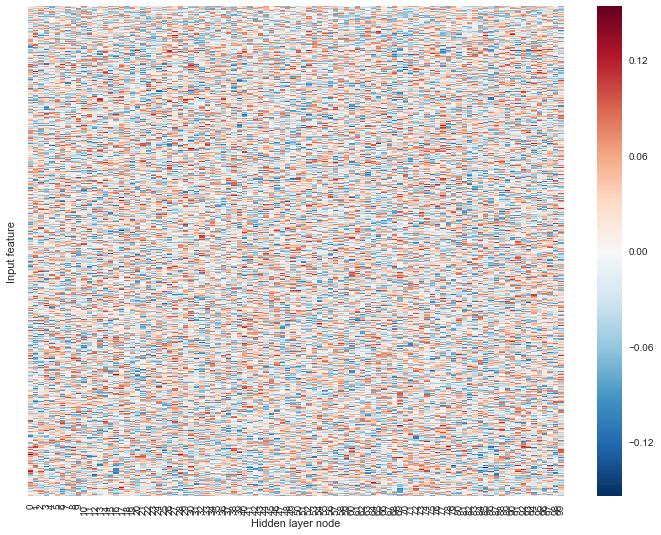
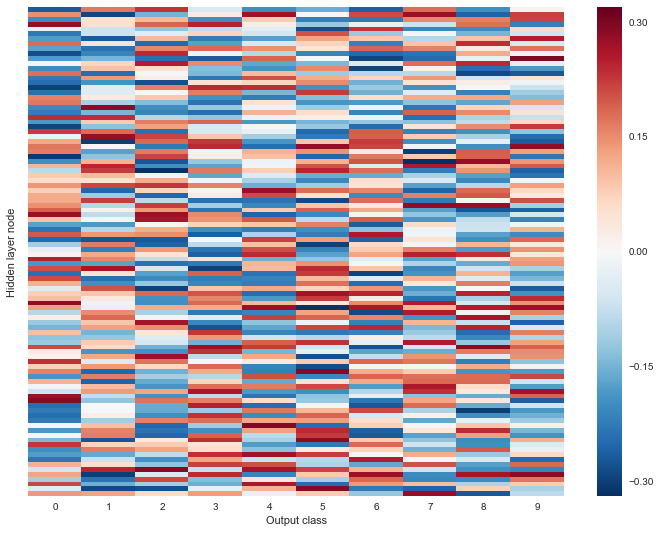
We next plotted the parameter weights of each layer. Unsurprisingly, the weights are all over the place.


TOP: weights of input to hidden layer;
BOTTOM: weights of hidden to output layer.
Visualizing the parameter weights across input features

When we visualize the parameter weights to the hidden layer by input feature, we find that some input features are more variable in terms of parameter weights than others.
Garson’s algorithm to calculate variable importance
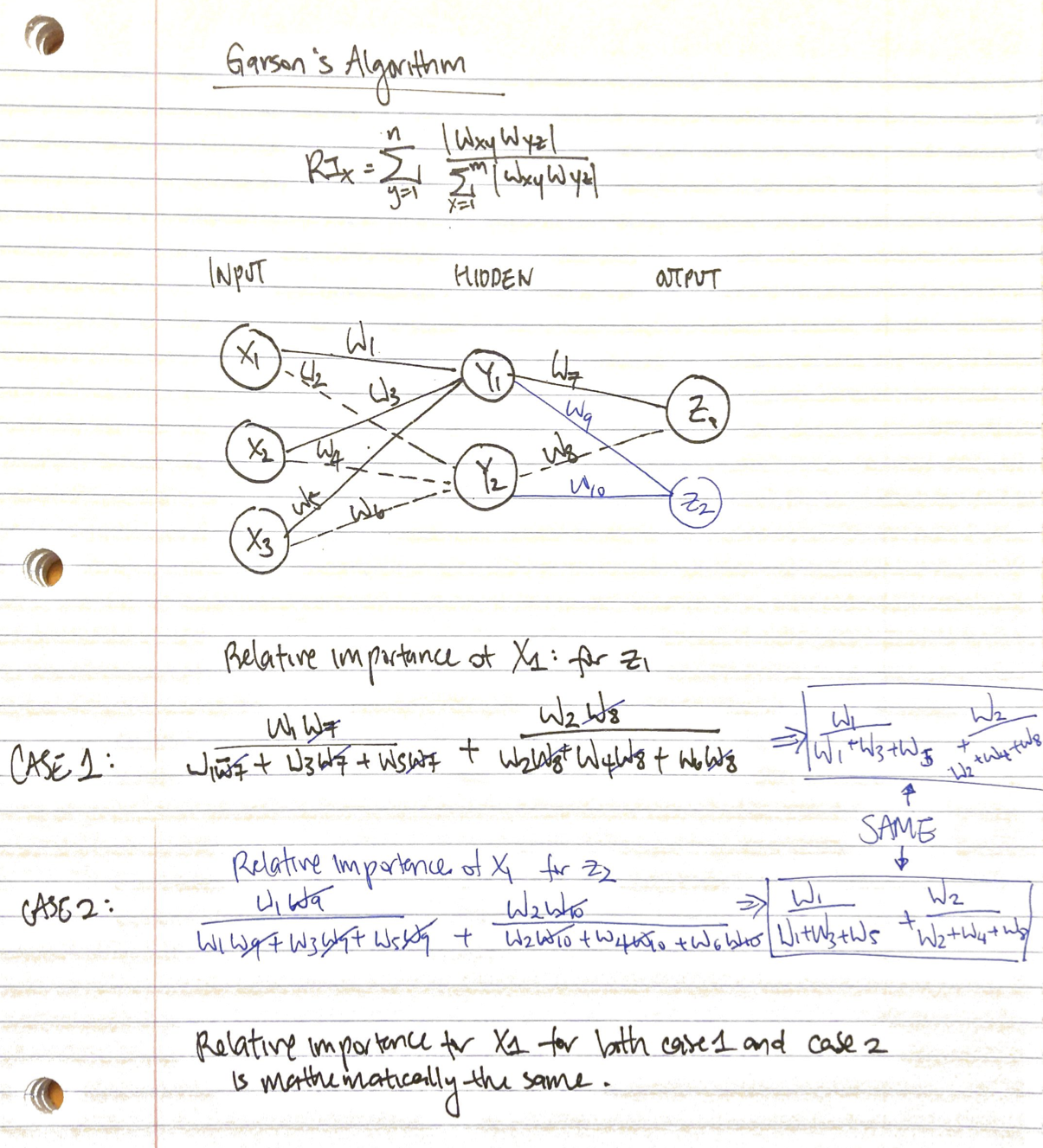
Using Garson’s algorithm to calculate the feature importance for each of the different output classes, we get the following figure…

… which shows the feature importance as being identical across the output classes. When we consider the math, this property makes sense:

Getting the important features
Finally, we are able to sort by the variable importance for the important features.
| relative_importance | |
|---|---|
| 69 | 0.001629 |
| 79 | 0.001550 |
| 502 | 0.001537 |
| 135 | 0.001526 |
| 530 | 0.001520 |
| 248 | 0.001511 |
| 417 | 0.001510 |
| 678 | 0.001506 |
| 401 | 0.001504 |
| 734 | 0.001495 |