I had a general understanding of Hidden Markov Models (HMM), but last week I wanted another explanation.
In my research, I came across Eddy. (2004). What is a hidden Markov model? Nature Biotechnology, 22(10):1315-1316. In it, there is a figure representing “A toy HMM for 5’ splice site recognition”:
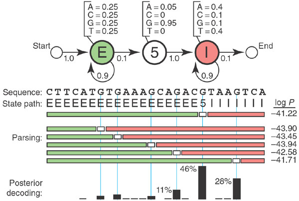
This figure shows a couple numbers i.e. -42.22 that I want to understand the calculation of.
Learning objective: By the end of the post, readers will be able to use transition and emission probabilities to calculate the state path probability for a given state path.
Terminology
In this example:
- the observe states are the 4 nucleotides:
A,T,G, andC - the hidden states are the 3 parts of a switch from exon (E) to intron (I):
E,5(for 5’ splice site), andI - the transition probability is the probability of changing from one hidden state to another (represented by the arrows in the the figure)
- the emission probability is the output probability of a hidden state (represented by the nucleotide output probability of a hidden state in the figure)
- the state path is the sequence of labels (e.g. E, 5, I) as we change from one state into another
- the state path probability is the probability of the state path and it is what we want to calculate
Calculation
We first setup the variables to describe the scenario.
nucleotides <- c("A", "C", "G", "T")
prob_emission <- list(
  "E" = setNames(rep(0.25, 4), nucleotides),
  "5" = setNames(c(0.05, 0, 0.95, 0), nucleotides),
  "I" = setNames(c(0.4, 0.1, 0.1, 0.4), nucleotides)
  )
prob_transition <- list(
  "^" = c("E"=1),
  "E" = c("E"=0.9, "5"=0.1),
  "5" = c("I"=1),
  "I" = c("I"=0.9, "$"=0.1)
  )

sequence   <- "CTTCATGTGAAAGCAGACGTAAGTCA"
state_path <- "EEEEEEEEEEEEEEEEEE5IIIIIII$"

## Reformat: string to character vector
sequence <- unlist(strsplit(sequence, ""))
state_path <- unlist(strsplit(state_path, ""))
We can then calculate the state path probability by multiplying the emission probability of the observed state with the transition probability of the current-to-next state.
prob <- as.numeric(prob_transition$`^`)
for (i in seq(1, length(sequence))){
  s0 <- state_path[[i]]
  s1 <- state_path[[i+1]]
  n <- sequence[i]

  e <- prob_emission[[s0]][[n]]
  t <- prob_transition[[s0]][[s1]]

  #' Product of probs of
  #' emission of observation and
  #' state transition from current state to next state
  prob <- prob * e * t
  }
This multiplication is done for the rest of the states in the sequence to get the state path probability of the state path. In total, 53 probabilities are multiplied together to get a probabilty of:
prob
## [1] 1.254647e-18
The log of this number is:
log(prob)
## [1] -41.21968
Thus giving us the -41.22 value shown in the figure.