Day09 - Mar 5, 2017
On Day02, I tried to implement a 2-layer fully connected neural network from scratch. Evaluation by Kaggle was 0.59330. Today I want to use neural networks from Scikit-learn to train a model for the Digit Recognizer Kaggle competition.
The Jupyter Notebook for this little project is found here.
Approach
- Train a neural network on 80% (n = 33,600)
- Validate on remaining 20% (n = 8,400)
- Submit predictions to Kaggle
In total there is 784 features and 42,000 training samples.
Neural Network / Multi-layer Perceptron classifier
from sklearn.neural_network import MLPClassifier

clf = MLPClassifier()
clf.fit(X_train, y_train)
The Scikit-learn documentation for the Multi-layer Perceptron classifier is found here. The MLPClassifier() arguments I use include:
alphawhich specifies the L2 penalty (regularization term) parameterhidden_layer_sizeswhich specifies the number of hidden layers and the number of nodes in each layerrandom_statewhich is a seed for the random number generator (ie. for reproducible results)
Specifying the hidden layer
In implementing a neural network, we need to specify the hidden layer (eg. How many layers? And how many nodes in each layer?). According to doug (2010):
In sum, for most problems, one could probably get decent performance (even without a second optimization step) by setting the hidden layer configuration using just two rules: (i) number of hidden layers equals one; and (ii) the number of neurons in that layer is the mean of the neurons in the input and output layers.
Thus our neural network is as follows:
- 1 input layer: 784 nodes (one node for each input feature)
- 1 hidden layer: 397 nodes (mean of 784 and 10)
- 1 output layer: 10 nodes (one for each output class)
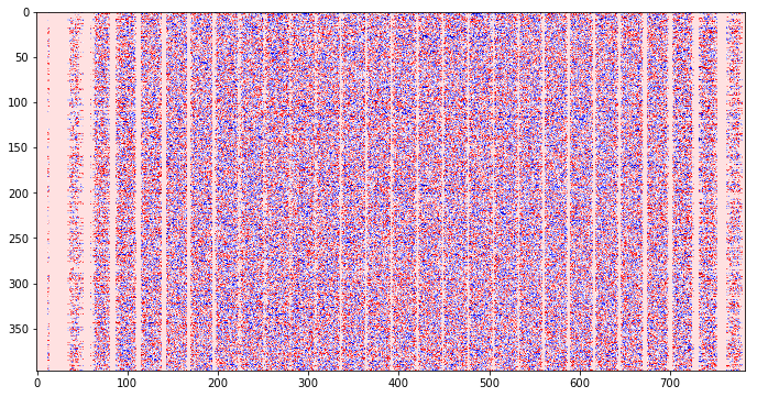
When we plot the weights between the nodes in the input (x-axis) and hidden (y-axis) layer, we find that some features are more informative than others.
Evaluation
Validating the model on the remaining part of the training data, we find the accuracy to be 96.5%. Submitting the predictions to Kaggle, the submission scored 0.96214 (which is an improvement on the previous score of 0.95871 using random forest).
Training on the whole set
When we retrain a new neural network on all data, the score improved to 0.96400 (+0.00529). When we counted the number of labels differing between the two sets of predictions, we have 1182 differences.
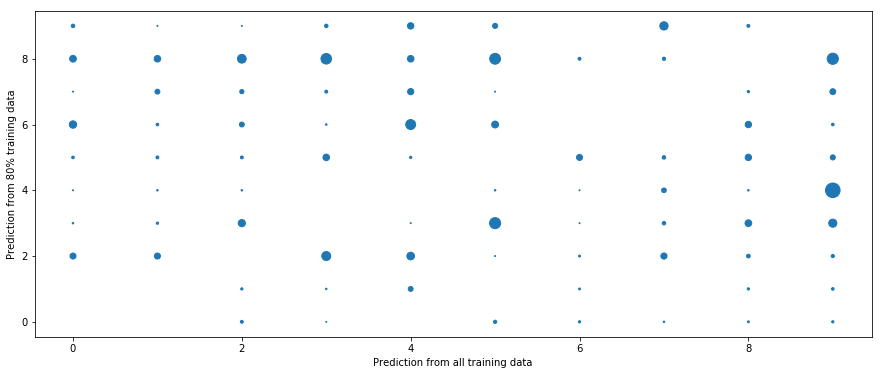
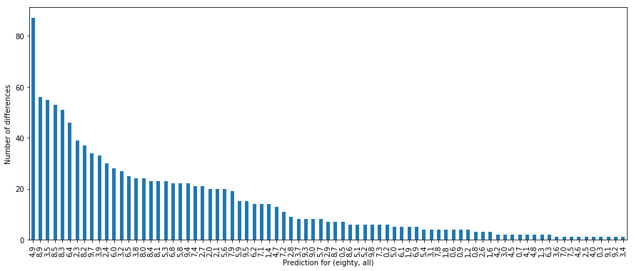
From the plots, we find that most inconsistent labels are between predicting 4 and 9. Understandable. Some people’s 4s look like 9s and 9s look like 4s. We also learn that training on all data is gives better performance than training on a portion of the data.