Today, I explore a new Kaggle data set:
- House Prices: Advanced Regression Techniques: Predict sales prices and practice feature engineering, RFs, and gradient boosting
The goal of this Kaggle competition is to predict the final price of each home from “79 explanatory variables describing (almost) every aspect of residential homes in Ames, Iowa.”
Index(['Id', 'MSSubClass', 'MSZoning', 'LotFrontage', 'LotArea', 'Street',
       'Alley', 'LotShape', 'LandContour', 'Utilities', 'LotConfig',
       'LandSlope', 'Neighborhood', 'Condition1', 'Condition2', 'BldgType',
       'HouseStyle', 'OverallQual', 'OverallCond', 'YearBuilt', 'YearRemodAdd',
       'RoofStyle', 'RoofMatl', 'Exterior1st', 'Exterior2nd', 'MasVnrType',
       'MasVnrArea', 'ExterQual', 'ExterCond', 'Foundation', 'BsmtQual',
       'BsmtCond', 'BsmtExposure', 'BsmtFinType1', 'BsmtFinSF1',
       'BsmtFinType2', 'BsmtFinSF2', 'BsmtUnfSF', 'TotalBsmtSF', 'Heating',
       'HeatingQC', 'CentralAir', 'Electrical', '1stFlrSF', '2ndFlrSF',
       'LowQualFinSF', 'GrLivArea', 'BsmtFullBath', 'BsmtHalfBath', 'FullBath',
       'HalfBath', 'BedroomAbvGr', 'KitchenAbvGr', 'KitchenQual',
       'TotRmsAbvGrd', 'Functional', 'Fireplaces', 'FireplaceQu', 'GarageType',
       'GarageYrBlt', 'GarageFinish', 'GarageCars', 'GarageArea', 'GarageQual',
       'GarageCond', 'PavedDrive', 'WoodDeckSF', 'OpenPorchSF',
       'EnclosedPorch', '3SsnPorch', 'ScreenPorch', 'PoolArea', 'PoolQC',
       'Fence', 'MiscFeature', 'MiscVal', 'MoSold', 'YrSold', 'SaleType',
       'SaleCondition', 'SalePrice'],
      dtype='object')
The Jupyter Notebook for this little project is found here.
Quantitative features
At a first pass (because it is simple and I want to get my hands on the data), we will only look at quantitative variables.
# Select quantitative variables (not including 'Id' and 'SalePrice')
features = train.columns[train.dtypes==int]
features = [f for f in features if f not in ["Id", "SalePrice"]]

X = train[features]
y = train["SalePrice"]
There is a total of 33 quantitative features (not including ‘Id’ and ‘SalePrice’).
Predicting sales price using Linear Regression
When I think of predicting a continuous-valued attribute, I think of regression. In particular, linear regression. In a simple (1 variable: x → y) case, this is drawing the line of best fit on a x-y scatter plot and using that line to predict for y from a new input x.
from sklearn.linear_model import LinearRegression
clf = LinearRegression()

from sklearn.model_selection import cross_val_score
scores = cross_val_score(clf, X, y, cv=3)

#> The scores: [ 0.84792899  0.78651395  0.69920021]
#> Accuracy: 0.78 (+/- 0.12)
Using the 33 quantitative features, the average accuracy of the cross-validation is 0.78.
Correlation of sales price
When we correlate the 33 quantitative features along with the sales price, we find that the overall quality is highly correlated with the sales price.
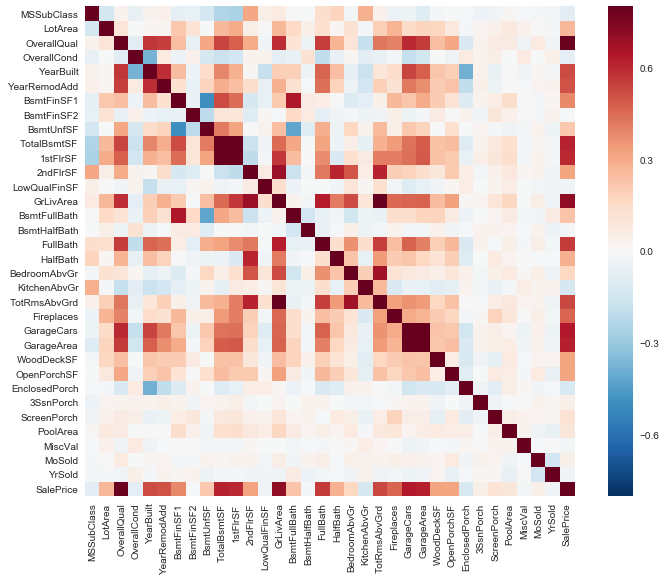
import seaborn as sns
corrmat = data.corr()
f, ax = plt.subplots(figsize=(12, 9))
sns.heatmap(corrmat, vmax=.8, square=True)
Looking at the overall quality
These plots further show that higher overall quality is indicative of higher sales prices.
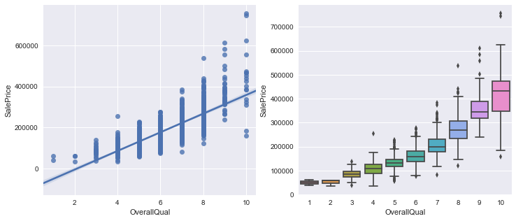
f, (ax1, ax2) = plt.subplots(figsize=(12, 5), ncols=2, nrows=1)
sns.regplot(x="OverallQual", y="SalePrice", data=data, ax=ax1)
sns.boxplot(x="OverallQual", y="SalePrice", data=data, ax=ax2)
# Predicting using only "OverallQual"
clf = LinearRegression()
scores = cross_val_score(clf, X[["OverallQual"]], y, cv=3)

#> The scores: [ 0.65298503  0.61625302  0.60493919]
#> Accuracy: 0.62 (+/- 0.04)
When we predict using only overall quality, the average accuracy of the CV is 0.62.
Predicting sales price using only highly correlated features
When we predict using only the “highly correlated features” (correlation magnitude with sales price above 0.25), the average accuracy of the CV is 0.77.
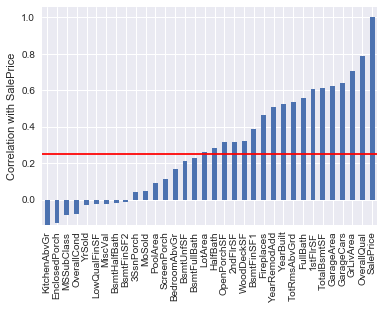
# Generate plot
df = pd.DataFrame(corrmat.SalePrice.sort_values())
df.plot.bar(legend=False)
plt.ylabel("Correlation with SalePrice")
plt.hlines(y=0.25, xmin=-10, xmax=100, color="red")

# Select the highly correlated features
highly_corr_features = corrmat.SalePrice.sort_values()
highly_corr_features = highly_corr_features[abs(highly_corr_features) > .25]
highly_corr_features = [f for f in highly_corr_features.index if f != 'SalePrice']
highly_corr_features
clf = LinearRegression()
scores = cross_val_score(clf, X[highly_corr_features], y, cv=3)

#> The scores: [ 0.84424068  0.77671438  0.69100392]
#> Accuracy: 0.77 (+/- 0.13)
Remarks
- Some features are highly correlated with the target variables, while others are not
- Using only highly correlated features is not enough to accurately predict the target variable